Functional ROI analyses of the HCP LANGUAGE Task Dataset
The demo uses the LANGUAGE task data in the Human Connectome Project (HCP) Young Adult dataset to showcase the funROI processing pipeline. It includes first-level processing, parcel generation, fROI definition, effect estimation, spatial correlation, and spatial overlap estimation.
The language localizer task in the HCP involves two conditions: a story condition, where participants listen to brief auditory stories followed by a comprehension question, and a math condition, where participants solve auditorily-presented arithmetic problems. These tasks are designed to activate distinct regions of the brain, with the story condition engaging the language network and the math condition serving as a non-linguistic control. Functional localization analyses of fMRI data collected during these tasks allow researchers to identify subject-specific brain regions involved in language processing.
Prerequisites
Before running the demo locally, please configure your AWS credentials to access the HCP dataset. Follow these steps:
Refer to this updated instruction for how to obtain AWS credentials for accessing the dataset.
Configure and store your credentials in the
~/.aws/credentialsfile. You can find detailed instructions in the AWS CLI user guide.Run the following code to download the data.
First Level Modeling
The first-level model in fMRI processing is designed to analyze individual subject data by modeling the relationship between task-related experimental conditions and the observed brain activity, by constructing a General Linear Model (GLM) for each voxel to estimate condition-specific effects.
The funROI toolbox wraps Nilearn’s first-level modeling, supporting event-related and block designs, customizable hemodynamic response functions, confound regression, and statistical contrasts. Below, we demonstrate how to configure and run a first-level model using funROI. For a list of customizable options for first level modeling, please refer to Nilearn first_level_from_bids. These options are supported for run_first_level using the toolbox.
In our analysis pipeline, we will run first-level modeling on two distinct samples:
N = 50 subjects for parcel generation
N = 10 subjects for fROI-based analyses
funROI is designed to operate on and generate data that is compliant with BIDS, the Brain Imaging Data Structure standard. For more information and additional resources on BIDS, please visit the official website at https://bids.neuroimaging.io/.
import funROI
funROI.set_bids_data_folder('./data/bids')
funROI.set_bids_preprocessed_folder('./data/bids')
funROI.set_bids_deriv_folder('./data/bids/derivatives')
funROI.set_analysis_output_folder("./data/analysis")

from funROI.first_level.nilearn import run_first_level
run_first_level(
    task = 'LANGUAGE',
    subjects = subjects1 + subjects2,
    space = 'MNINonLinear',
    contrasts = [
        ('story', {'story': 1}),
        ('math', {'math': 1}),
        ('story-math', {'story': 1, 'math': -1}),
        ('math-story', {'math': 1, 'story': -1})
    ],
    hrf_model='spm + derivative',
    smoothing_fwhm=4,
    noise_model="ar1",
    slice_time_ref = 0
)
Generate Parcels for the Language System
In this section, we’re focusing on parcel generation using the group-constrained, subject-specific (GcSS) approach introduced by Fedorenko et al (2010).
The process starts by generating a probabilistic map by overlaying individual activation/contrast maps obtained from a localizer contrast. The map shows what % of the participants had significant activation/contrast value at each voxel.
We then apply a watershed algorithm to segment this probabilistic map into parcels (brain masks). These parcels can later be used as spatial constraints for defining individual fROIs. When generating the parcels with the toolbox, you can customize the spatial smoothing applied to the probabilistic map, the minimum voxel probability required for inclusion in parcels, and the parcel-level thresholding parameters—including the minimum voxel size and the minimum proportion of subjects that must have a significant voxel with respect to the localizer contrast within that parcel.
Refer to the ParcelsGenerator documentation for more details.
In this part, we will demonstrate how to generate parcels for the language system using a sample of 50 subjects. We will focus on the story-math contrast to isolate regions of the brain involved in language processing.
from funROI.analysis import ParcelsGenerator
parcels_generator = ParcelsGenerator(
    parcels_name="Language",
    smoothing_kernel_size=10,
    overlap_thr_vox=0.15,
)
parcels_generator.add_subjects(
    subjects=subjects1,
    task="LANGUAGE",
    contrasts=["story-math"],
    p_threshold_type="none",
    p_threshold_value=0.05,
)
parcels = parcels_generator.run()
Let’s take a look at the parcels generated:
plot_mni152_surface_roi_map(
    parcels,
    output_file_prefix="output_language_parcels",
    threshold=1.,
    vmin=1.,
    vmax=np.max(parcels.get_fdata())
)
display(Image("output_language_parcels.png"))
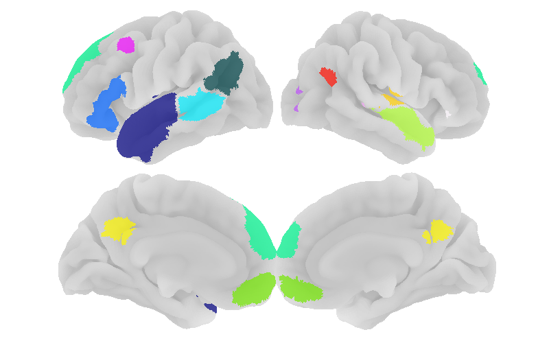
Empirically, we know that smaller parcels are often non-robust, meaning that they might be an artifact of an insufficiently large number of participants. We can filter the parcels by size:
parcels = parcels_generator.filter(min_voxel_size=100)
Let’s visualize the resulting parcels:
parcel_ids = np.unique(parcels.get_fdata())
parcel_ids = parcel_ids[parcel_ids != 0]

n = len(parcel_ids)
ncols = 3
nrows = int(np.ceil(n / ncols))

fig, axes = plt.subplots(
    nrows, ncols,
    figsize=(4 * ncols, 2 * nrows)
)

axes = np.atleast_1d(axes).ravel()

for ax, parcel in zip(axes, parcel_ids):
    img_parcel = new_img_like(
        parcels,
        (parcels.get_fdata() == parcel).astype(int)
    )

    plot_roi(
        img_parcel,
        display_mode="ortho",
        draw_cross=False,
        axes=ax,
        annotate=False,
        colorbar=False
    )
    ax.set_title(f"ROI {int(parcel)}", fontsize=10)
/var/folders/k0/md38zs8x1395ywbtngppz3k00000gp/T/ipykernel_59606/3216352333.py:16: UserWarning: Data array used to create a new image contains 64-bit ints. This is likely due to creating the array with numpy and passing `int` as the `dtype`. Many tools such as FSL and SPM cannot deal with int64 in Nifti images, so for compatibility the data has been converted to int32.
  img_parcel = new_img_like(
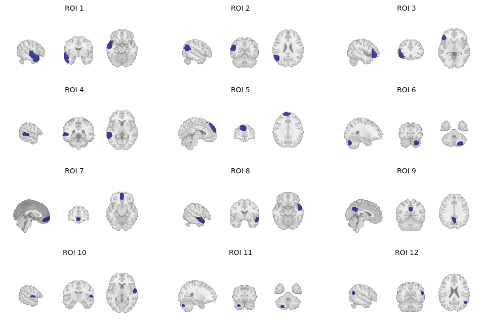
Other toolbox options include filtering by % of subjects that show significant activation in that parcel.
Define Language fROIs for Individual Subjects
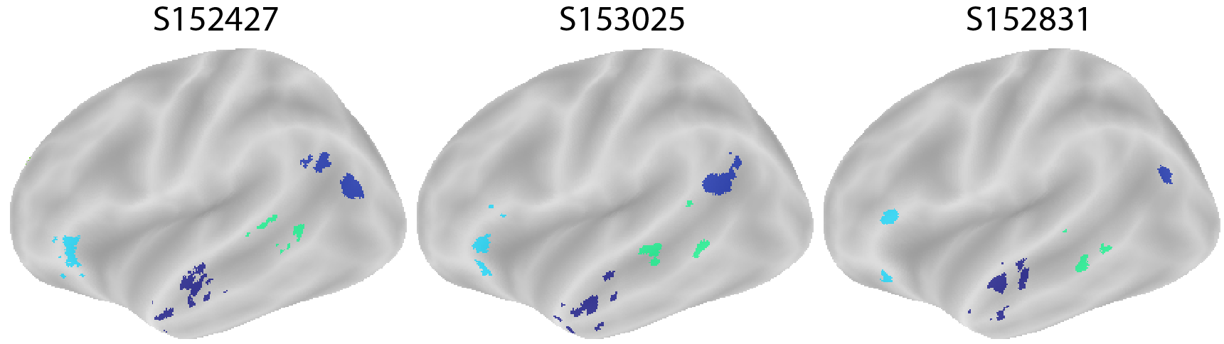
For each parcel generated in the previous step, we now define subject-specific functional regions of interest (fROIs) for the language system. Within each parcel, the language fROI for a subject is defined as the top 10% of voxels that exhibit the strongest story-math contrast.
If you proceed directly to the analyses with fROI definition configuration provided, the subject fROIs are automatically defined and saved in the BIDS derivatives. You can customize the definition of the fROI by specifying the proportion of the parcel size (e.g., 10%), a fixed number of voxels, or a significance threshold with respect to a given p-value. The following example demonstrates how to manually generate and inspect fROIs.
Let’s inspect the first three subjects in sample 2 to look at their language fROIs:
from funROI.analysis import FROIGenerator
parcels_config = funROI.ParcelsConfig.from_analysis_output(
    "Language",
    smoothing_kernel_size=10,
    overlap_thr_vox=0.15,
    overlap_thr_roi=0,
    min_voxel_size=100
)
froi = funROI.FROIConfig(
    task="LANGUAGE",
    contrasts=["story-math"],
    threshold_type="percent",
    threshold_value=0.1,
    parcels=parcels_config
)
froi_generator = FROIGenerator(subjects2[:3], froi)
froi_imgs = froi_generator.run()
for subject_label, froi_img in froi_imgs:
    plot_mni152_surface_roi_map(
        froi_img,
        inflate=True,
        output_file_prefix=f"output_froi_{subject_label}",
        threshold=1.,
        vmin=1.,
        vmax=np.max(froi_img.get_fdata())
    )
display(Image("output_frois.png"))
Analysis: Effect Sizes
Effect size estimation is a critical step in fROI analysis, as it provides a quantitative measure of the strength of the neural response to specific contrasts or conditions.
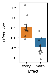
In this section, we will demonstrate how to estimate effect sizes for story and math conditions within subjects’ language fROIs. The effect sizes of the language system will be evaluated in the fROIs defined in the previous section. Separate fMRI runs are used to define the fROIs and to estimate effect sizes, to avoid double dipping.
We are using the 10-subject independent sample, separate from the set of subjects that we used to define the parcels (as described previously). Here and in later plots, each dot represents a subject.
from funROI.analysis import EffectEstimator
effect_estimator = EffectEstimator(subjects=subjects2, froi=froi)
df_summary, df_detail = effect_estimator.run(
    task="LANGUAGE", effects=["story", "math"])
As we examine the effect sizes for the subjects’ language system, we observe the expected higher responses to story compared to math. This confirms the validity of our approach.
plt.figure(figsize=(2,3), tight_layout=True)
data = df_summary.groupby(["subject", "effect"]).mean().reset_index()
sns.barplot(data=data, y="size", x="effect", hue="effect", errorbar="se",
            order=["story", "math"])
sns.stripplot(data=data, y="size", x="effect", dodge=False, alpha=0.5,
              jitter=True, order=["story", "math"], color='black')
plt.ylabel("Effect Size")
plt.xlabel("Effect")
Text(0.5, 0, 'Effect')
We can examine responses in individual fROIs. We see substantial heterogeneity in response magnitudes to each task, due likely to a combination of physiological and cognitive factors:
plt.figure(figsize=(8, 4), tight_layout=True)
sns.barplot(data=df_summary, y="size", x="froi", hue="effect", errorbar="se",
           hue_order=["story", "math"])
sns.stripplot(data=df_summary, y="size", x="froi", hue="effect", dodge=True,
              alpha=0.5, jitter=True, hue_order=["story", "math"],
              color='black', legend=False)
plt.ylabel("Effect Size")
plt.xlabel("fROI")
plt.legend(loc='upper left', title='Effect', bbox_to_anchor=(1, 1))
/var/folders/k0/md38zs8x1395ywbtngppz3k00000gp/T/ipykernel_59606/1787390042.py:4: FutureWarning:

Setting a gradient palette using color= is deprecated and will be removed in v0.14.0. Set `palette='dark:black'` for the same effect.

  sns.stripplot(data=df_summary, y="size", x="froi", hue="effect", dodge=True,
<matplotlib.legend.Legend at 0x38ab7bdf0>
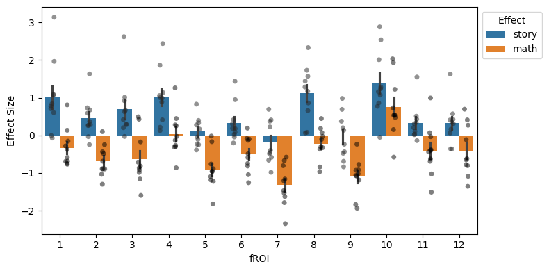
Research note: in this example, the heterogeneity we observe is largely due to the fact that the HCP language localizer is very imprecise. A story>math contrast includes many different cognitive processes other than language (e.g., situation modeling to accurately track a narrative and social reasoning to interpret the characters’ intent). Thus, not all fROIs are language-specific (which is something we can test by estimating these fROIs’ responses to other conditions and tasks).
Analysis: Spatial Correlation Across Conditions
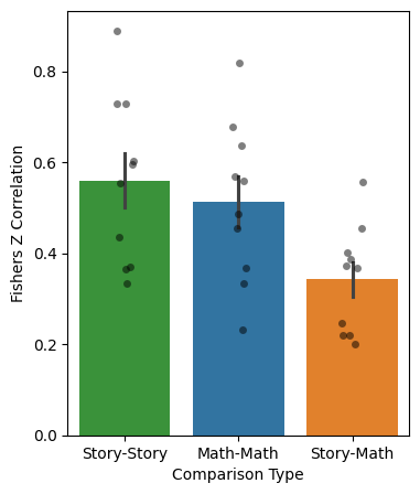
Spatial correlation provides a valuable metric for assessing the similarity of within-subject activation patterns across different conditions or runs, allowing researchers to evaluate the consistency of functional responses in specific regions of the brain. This analysis can be performed on either parcels or fROIs.
Here, we will estimate the spatial correlation between the story and math conditions within each language parcel (using the parcels defined in the “Generate Parcels for the Language System” section).
from funROI.analysis import SpatialCorrelationEstimator
spcorr_estimator = SpatialCorrelationEstimator(
    subjects=subjects2,
    froi=parcels_config
)
df_math, _ = spcorr_estimator.run(
    task1='LANGUAGE', effect1='math', task2='LANGUAGE', effect2='math',
)
df_story, _ = spcorr_estimator.run(
    task1='LANGUAGE', effect1='story', task2='LANGUAGE', effect2='story',
)
df_between, _ = spcorr_estimator.run(
    task1='LANGUAGE', effect1='story', task2='LANGUAGE', effect2='math',
)
Let’s visualize the results:
df_math['Type'] = 'Math-Math'
df_story['Type'] = 'Story-Story'
df_between['Type'] = 'Story-Math'
data = pd.concat(
    [df_between, df_math, df_story]
).groupby(["subject", "Type"]).mean().reset_index()

plt.figure(figsize=(4,5))
sns.barplot(data=data, y="fisher_z", x="Type", hue="Type", errorbar="se",
            order=["Story-Story",  "Math-Math", "Story-Math"])
sns.stripplot(data=data, y="fisher_z", x="Type", dodge=False, alpha=0.5,
              jitter=True, order=["Story-Story",  "Math-Math", "Story-Math"],
              color='black')
plt.ylabel("Fishers Z Correlation")
plt.xlabel("Comparison Type")
Text(0.5, 0, 'Comparison Type')
Analysis: Overlap Between fROIs
Assessing the spatial overlap between parcels or fROIs can be useful in various ways, guiding comparisons across tasks and conditions. In this section, we showcase an example of computing the degree of overlap between the language system defined using the localizer, as stated above (10% top voxels), across subjects and within subjects using different runs.
We support two overlap measurements: Dice coefficient and overlap coefficient. The default is the overlap coefficient, which is what we will use now.
from funROI.analysis import OverlapEstimator
overlap_estimator = OverlapEstimator()
data = []
for i, subject1 in enumerate(subjects2):
    df, _ = overlap_estimator.run(
        froi1=froi, froi2=froi, subject1=subject1, subject2=subject1,
        run1='01', run2='02'
    )
    data.append(df[df['froi1'] == df['froi2']])

    subject2 = subjects2[(i+1) % len(subjects2)]
    df, _ = overlap_estimator.run(
        froi1=froi, froi2=froi, subject1=subject1, subject2=subject2,
        run1='01', run2='02'
    )
    data.append(df[df['froi1'] == df['froi2']])

data = pd.concat(data)
The results visualized below illustrate the spatial overlap results:
data.loc[data['subject1'] == data['subject2'], 'Type'] = 'Within'
data.loc[data['subject1'] != data['subject2'], 'Type'] = 'Between'
data_mean = data.groupby(["subject1", "subject2", "Type"]).mean().reset_index()
plt.figure(figsize=(2,3), tight_layout=True)
sns.barplot(data=data_mean, y="overlap", x="Type", hue="Type", errorbar="se")
sns.stripplot(data=data_mean, y="overlap", x="Type", dodge=False,
              alpha=0.5, jitter=True, color='black')
plt.ylabel("Overlap")
plt.xlabel("Comparison Type")
Text(0.5, 0, 'Comparison Type')
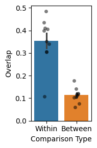
They demonstrate that the fROIs from the same subject (defined using different sets of data) are more consistent compared to fROIs from different subjects, a result that motivates the entire subject-specific fROI approach to fMRI analyses.
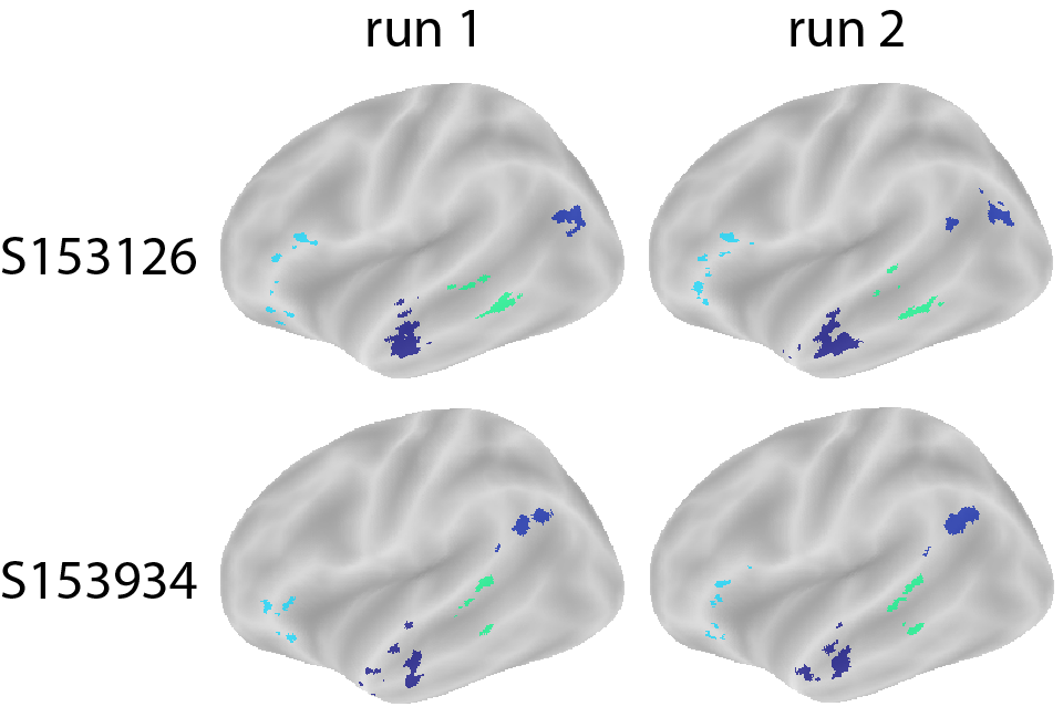
Let’s see some example fROIs by leveraging the fROI generator:
Two brains in the same row: fROI defined for the same subject across different runs.
Two brains in the same column: fROIs defined for different subjects.
from funROI.analysis import FROIGenerator
for subject, run in zip(['153126', '153126', '153934', '153934'],
                        ['01', '02', '01', '02']):
    froi_generator = FROIGenerator([subject], froi, run_label=run)
    froi_imgs = froi_generator.run()
    subject_label, froi_img = froi_imgs[0]
    plot_mni152_surface_roi_map(
        froi_img,
        inflate=True,
        output_file_prefix=f"output_froi_{subject_label}_run{run}",
        threshold=1.,
        vmin=1.,
        vmax=np.max(froi_img.get_fdata())
    )
display(Image("output_frois_comparison.png"))
Analysis: Laterality Index
The human language network is typically left-lateralized, with stronger and more spatially reliable responses in the left hemisphere than in the right hemisphere. This left-lateralized fronto-temporal system is commonly identified with individual-subject functional localizers. Here, we ask whether the language fROIs defined from the HCP LANGUAGE task show the same expected leftward bias.
from funROI.analysis import LateralityIndexAnalyzer
li_analyzer = LateralityIndexAnalyzer(
    subjects=subjects2,
    froi=funROI.FROIConfig(
        task="LANGUAGE",
        contrasts=["story-math"],
        threshold_type="none",
        threshold_value=0.05,
        parcels="none"
        )
)
df_li = li_analyzer.run()
df_li = df_li.sort_values(by="laterality_index", ascending=False)
plt.figure(figsize=(4,3), tight_layout=True)
sns.barplot(data=df_li, y="laterality_index", x="subject", hue="subject")
plt.ylabel("Laterality Index")
plt.xlabel("Subject")
plt.xticks(rotation=90)
plt.show()
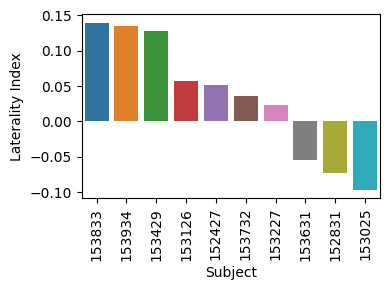
We observe mostly positive laterality indices, indicating stronger left- than right-hemisphere language activation in this sample!
Analysis: Functional Connectivity Between the Language and MD Networks
We next examine functional connectivity among fROIs. In addition to the language network, we define parcels for the multiple-demand (MD) network: a domain-general fronto-parietal system associated with effortful cognitive control and task demands. In the HCP LANGUAGE task, the math > story contrast provides a useful contrast for identifying MD-responsive regions.
Prior work has shown that the language and MD systems are functionally dissociable: regions within the same network tend to show stronger correlated BOLD fluctuations than regions across the language and MD networks. Blank, Kanwisher, and Fedorenko (2014) specifically report this dissociation using patterns of BOLD signal fluctuations. We therefore expect stronger connectivity within language fROIs and within MD fROIs than between language and MD fROIs.
We first define MD parcels using the math > story contrast:
from funROI.analysis import ParcelsGenerator
parcels_generator = ParcelsGenerator(
    parcels_name="MD",
    smoothing_kernel_size=10,
    overlap_thr_vox=0.15,
    min_voxel_size=100
)
parcels_generator.add_subjects(
    subjects=subjects1,
    task="LANGUAGE",
    contrasts=["math-story"],
    p_threshold_type="none",
    p_threshold_value=0.05,
)
parcels = parcels_generator.run()
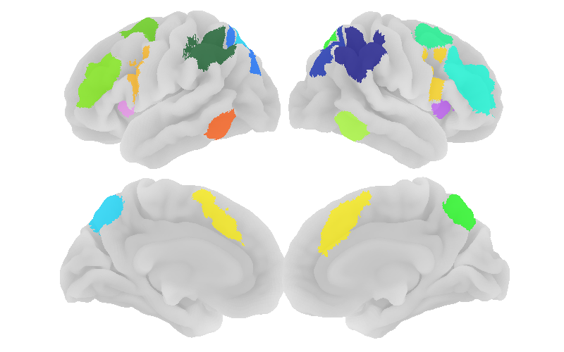
The resulting MD parcels are shown below:
plot_mni152_surface_roi_map(
    parcels,
    output_file_prefix="output_MD_parcels",
    threshold=1.,
    vmin=1.,
    vmax=np.max(parcels.get_fdata())
)

display(Image("output_MD_parcels.png"))
We then compute three classes of functional connectivity: connectivity among language fROIs, connectivity among MD fROIs, and connectivity between language and MD fROIs.
from funROI.analysis import FunctionalConnectivityEstimator
froi_lang = funROI.FROIConfig(
    task="LANGUAGE",
    contrasts=["story-math"],
    threshold_type="percent",
    threshold_value=0.1,
    parcels=funROI.ParcelsConfig.from_analysis_output(
        "Language",
        smoothing_kernel_size=10,
        overlap_thr_vox=0.15,
        overlap_thr_roi=0,
        min_voxel_size=100
    )
)

froi_md = funROI.FROIConfig(
    task="LANGUAGE",
    contrasts=["math-story"],
    threshold_type="percent",
    threshold_value=0.1,
    parcels=funROI.ParcelsConfig.from_analysis_output(
        "MD",
        smoothing_kernel_size=10,
        overlap_thr_vox=0.15,
        overlap_thr_roi=0,
        min_voxel_size=100
    )
)

data = []
for comparison, froi1, froi2 in zip(
    ['Language-Language', 'MD-Language', 'MD-MD'],
    [froi_lang, froi_md, froi_md],
    [froi_lang, froi_lang, froi_md]
    ):
    df_summary, _ = FunctionalConnectivityEstimator(
        subjects = subjects2, froi1 = froi1, froi2 = froi2,
    ).run(
        task="LANGUAGE", space="MNINonLinear",
        froi1_run_label='odd',
        froi2_run_label='odd',
        run_filter='even',
    )
    df_summary['Comparison'] = comparison
    data.append(df_summary)
data = pd.concat(data)
data['froi1'] = data['Comparison'].apply(lambda x: x.split('-')[0]) + '_' + data['froi1'].astype(str)
data['froi2'] = data['Comparison'].apply(lambda x: x.split('-')[1]) + '_' + data['froi2'].astype(str)
data_avg = data.groupby(["froi1", "froi2", "Comparison"])['fisher_z'].mean().reset_index()
data_avg = data_avg[data_avg['froi1'] != data_avg['froi2']]

order = lambda x: (x[0], int(x.split('_')[1]))
data_pivot = data_avg.pivot(index='froi1', columns='froi2', values='fisher_z')
data_pivot = data_pivot.reindex(index=sorted(data_pivot.index, key=order),
                                columns=sorted(data_pivot.columns, key=order))
plt.figure(figsize=(10, 8))
sns.heatmap(data_pivot, annot=False, center=0, cmap='coolwarm',
            mask=np.triu(np.ones(data_pivot.shape)),
            cbar_kws={'label': 'Fisher Z'})
plt.xlabel("fROI 2")
plt.ylabel("fROI 1")
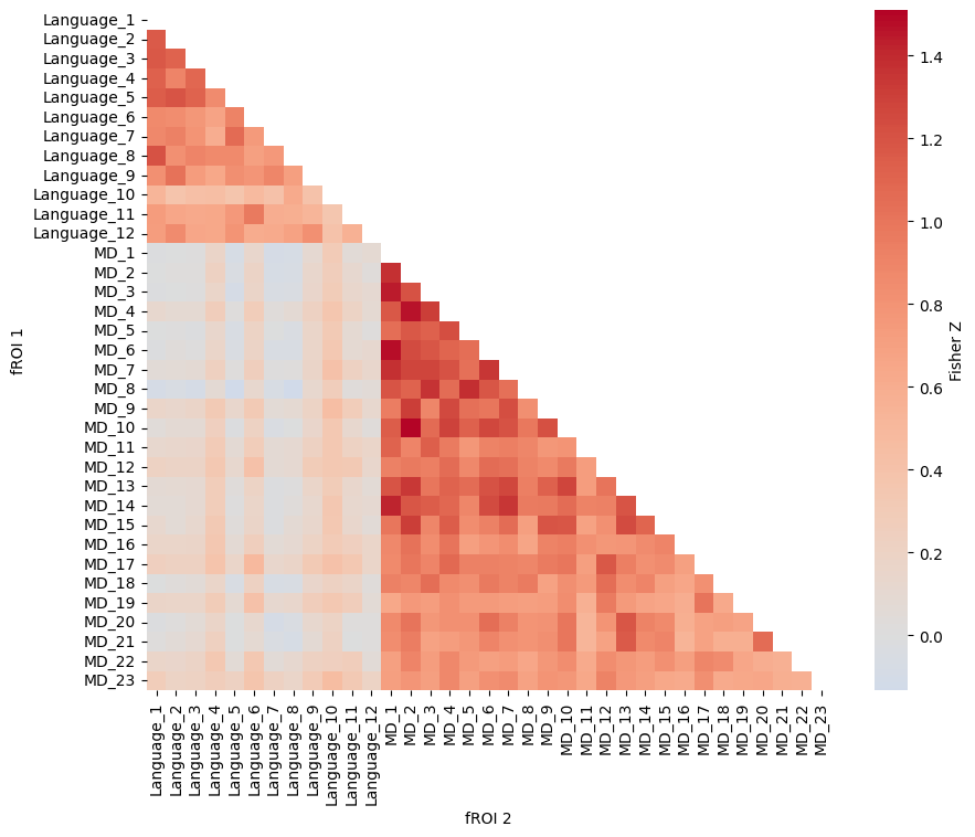
As expected, within-network connectivity is stronger than between-network connectivity: language fROIs are more strongly connected to other language fROIs, and MD fROIs are more strongly connected to other MD fROIs, than language and MD fROIs are to each other. This pattern is consistent with the view that the language and MD networks are spatially adjacent but functionally dissociable systems.
In this demo, we showcased a complete workflow for analyzing the language system in the HCP dataset, starting with first-level modeling and culminating in subject-specific fROI definitions derived from the story>math contrast. By constructing probabilistic maps, generating parcels, and selecting subject-specific peak activation voxels within these parcels, we demonstrated how to obtain robust measures of functional responses. We then evaluated these fROIs through a series of analyses—including effect size estimation, spatial correlation, overlap assessment, laterality index estimation, and functional connectivity analyses—showing that subject-specific fROIs exhibit expected properties of the language system, including stronger responses to stories than math, left-lateralized activation, and stronger within-network than between-network connectivity. Overall, this pipeline highlights the benefits of a tailored fROI approach for capturing individual differences in language-related brain activity.